Statistics One (Coursera)

Assignment:4

Assignment 4 deadline got over today. So i am putting the assignment 4 questions and answers here. Hope it will help others to solve the questions. 

setwd("  ")

library(psych)

PE=read.table("Stats1.13.HW.04.txt",header = T)

describe(PE)

#Question1: What is the correlation between salary and years of professional experience?

cor(PE[2:4])

round(cor(PE[2:4]),2)

           salary     years   courses

salary  1.0000000 0.7448961 0.5410249

years   0.7448961 1.0000000 0.3336635

courses 0.5410249 0.3336635 1.0000000

> round(cor(PE[2:4]),2)

        salary years courses

salary    1.00  0.74    0.54

years     0.74  1.00    0.33

courses   0.54  0.33    1.00

#Question2: What is the correlation between salary and courses completed?

round(cor(PE$salary, PE$courses),2)

[1] 0.54

#Question3: What is the percentage of variance explained in a regression model with salary as the outcome variable and professional experience as the predictor variable?

model1=lm(PE$salary ~ PE$years)

summary(model1)

Call:

lm(formula = PE$salary ~ PE$years)

Residuals:

     Min       1Q   Median       3Q      Max 

-21356.2  -5290.8    257.5   4797.1  20298.9 

Coefficients:

            Estimate Std. Error t value Pr(>|t|)    

(Intercept)  32810.3     2763.4   11.87   <2e-16 font="">

PE$years      5637.8      358.9   15.71   <2e-16 font="">

---

Signif. codes:  0 ‘***’ 0.001 ‘**’ 0.01 ‘*’ 0.05 ‘.’ 0.1 ‘ ’ 1

Residual standard error: 7457 on 198 degrees of freedom

Multiple R-squared:  0.5549, Adjusted R-squared:  0.5526 

F-statistic: 246.8 on 1 and 198 DF,  p-value: < 2.2e-16

#Question4: Compared to the model from Question 3, would a regression model predicting salary from the number of courses be considered a better fit to the data?

model2=lm(PE$salary ~ PE$courses)

summary(model2)

Call:

lm(formula = PE$salary ~ PE$courses)

Residuals:

   Min     1Q Median     3Q    Max 

-23472  -5474   -615   6031  37828 

Coefficients:

            Estimate Std. Error t value Pr(>|t|)    

(Intercept) 62719.43    1553.18  40.381   <2e-16 font="">

PE$courses    716.09      79.11   9.052   <2e-16 font="">

---

Signif. codes:  0 ‘***’ 0.001 ‘**’ 0.01 ‘*’ 0.05 ‘.’ 0.1 ‘ ’ 1

Residual standard error: 9400 on 198 degrees of freedom

Multiple R-squared:  0.2927, Adjusted R-squared:  0.2891 

F-statistic: 81.94 on 1 and 198 DF,  p-value: < 2.2e-16

#Question5: Now let's include both predictors (years of professional experience and courses completed) in a regression model with salary as the outcome. Now what is the percentage of variance explained?

model3=lm(PE$salary ~ PE$years + PE$courses)

summary(model3)

Call:

lm(formula = PE$salary ~ PE$years + PE$courses)

Residuals:

     Min       1Q   Median       3Q      Max 

-17788.6  -4761.9    -66.1   4174.6  19556.4 

Coefficients:

            Estimate Std. Error t value Pr(>|t|)    

(Intercept) 31362.90    2460.46  12.747  < 2e-16 ***

PE$years     4806.65     337.86  14.227  < 2e-16 ***

PE$courses    435.62      59.09   7.373 4.52e-12 ***

---

Signif. codes:  0 ‘***’ 0.001 ‘**’ 0.01 ‘*’ 0.05 ‘.’ 0.1 ‘ ’ 1

Residual standard error: 6619 on 197 degrees of freedom

Multiple R-squared:  0.6511, Adjusted R-squared:  0.6476 

F-statistic: 183.8 on 2 and 197 DF,  p-value: < 2.2e-16

#Question6: What is the standardized regression coefficient for years of professional experience, predicting salary?

model1.z=lm(scale(PE$salary) ~ scale(PE$years))

summary(model1.z)

Call:

lm(formula = scale(PE$salary) ~ scale(PE$years))

Residuals:

    Min      1Q  Median      3Q     Max 

-1.9155 -0.4745  0.0231  0.4303  1.8207 

Coefficients:

                  Estimate Std. Error t value Pr(>|t|)    

(Intercept)     -1.460e-16  4.730e-02    0.00        1    

scale(PE$years)  7.449e-01  4.741e-02   15.71   <2e-16 font="">

---

Signif. codes:  0 ‘***’ 0.001 ‘**’ 0.01 ‘*’ 0.05 ‘.’ 0.1 ‘ ’ 1

Residual standard error: 0.6689 on 198 degrees of freedom

Multiple R-squared:  0.5549, Adjusted R-squared:  0.5526 

F-statistic: 246.8 on 1 and 198 DF,  p-value: < 2.2e-16

#Question7: What is the standardized regression coefficient for courses completed, predicting salary?

model2.z=lm(scale(PE$salary) ~ scale(PE$courses))

summary(model2.z)

Call:

lm(formula = scale(PE$salary) ~ scale(PE$courses))

Residuals:

    Min      1Q  Median      3Q     Max 

-2.1052 -0.4910 -0.0552  0.5409  3.3929 

Coefficients:

                    Estimate Std. Error t value Pr(>|t|)    

(Intercept)       -1.663e-16  5.962e-02   0.000        1    

scale(PE$courses)  5.410e-01  5.977e-02   9.052   <2e-16 font="">

---

Signif. codes:  0 ‘***’ 0.001 ‘**’ 0.01 ‘*’ 0.05 ‘.’ 0.1 ‘ ’ 1

Residual standard error: 0.8431 on 198 degrees of freedom

Multiple R-squared:  0.2927, Adjusted R-squared:  0.2891 

F-statistic: 81.94 on 1 and 198 DF,  p-value: < 2.2e-16

#Question8: What is the mean of the salary distribution predicted by the model including both years of professional experience and courses completed as predictors? (with 0 decimal places)

data.predicted = fitted(model3)

mean(data.predicted)

[1] 75426.44

#Question9: What is the mean of the residual distribution for the model predicting salary from both years of professional experience and courses completed? (with 0 decimal places)

PE$e=resid(model3)

mean(PE$e)

[1] -1.893208e-14

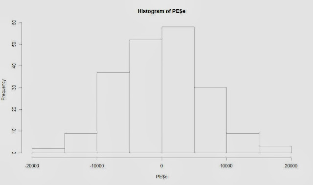
#Question10: Are the residuals from the regression model with both predictors normally distributed?

hist(PE$e)

Thanks for viewing...:-)